We give a code for drawing parallel level plots of the clusters. The clustering algorithms are provided by R. First generate the data and list the clustering algorithms.
dendat<-sim.data(n=300,seed=5,type="mulmod")
algos<-c("kmeans","single","complete","average",
"ward","mcquitty","median","centroid")
Draw the parallel level plot.
algo<-algos[3]   # choose the algorithm
k<-4             # choose the number of clusters
paraclus(dendat,algo=algo,k=k)  # draw the plot
We give a code for drawing graphical matrices with the permutation given by the clusters. First we generate the data.
dendat<-sim.data(n=300,seed=5,type="cross")
We use hierarchical clustering.
dis<-dist(dendat)
hc<-hclust(dis, method=algos[3])
classes=cutree(hc,k=4)
permu<-order(classes)
graph.matrix(dendat,permu=permu,col=classes)

plot(dendat,col=classes) # scatter plot
We use the k-means algorithm.
cl<-kmeans(dendat,centers=4)
classes<-cl$cluster
permu<-order(classes)
graph.matrix(dendat,permu=permu,col=classes)

plot(dendat,col=classes) # scatter plot
Graphical matrix of tail clusters.
rho<-0.55
tt<-leafsfirst(dendat=dendat,rho=rho)
graph.matrix(dendat,tt=tt)

colo<-tree.segme(tt,paletti=seq(1,1000))
plot(dendat,col=colo)
First generate the data.
dendat<-sim.data(n=300,seed=5,type="cross")
Perform hierarchical clustering.
dis<-dist(dendat)
hc<-hclust(dis, method=algos[3])
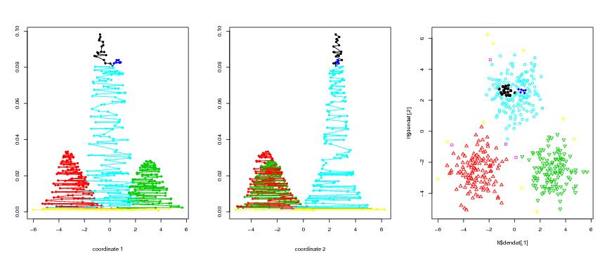
Transform the herarchical clustering tree to a tree generating a branching curve, and then make a parallel level plot of the tree.
tr<-dend2parent(hc,dendat)
plotbary(tr,coordi=2,colometh="cluster",colothre=3)

plot(hc, hang = -1)  # plot also the dendrogram
We give the code for reproducing this figure. First generate the data.
dendat<-sim.data(n=n,type="nested",seed=1)
Calculate a kernel estimate, calculate a level set tree of the kernel estimate, and calculate the likelhood tree.
ke<-pcf.kern(dendat,h=1,N=c(64,64)) # kernel estimate
lst<-leafsfirst(ke)                 # level set tree
lt<-liketree(dendat,ke,lst)         # likelihood tree
We visualize the likelihood tree with a parallel plot.
plotbary(lt,coordi=1) # coordi=1 or coordi=2
In the 2D case one may also draw the colored scatter plot
dendat.sub<-lt$denda      # subsetting
paletti<-c("red","blue","green",
 "orange","navy","darkgreen",
 "orchid","aquamarine","turquoise",
 "pink","violet","magenta","chocolate","cyan",
 colors()[50:657],colors()[50:657])
col<-colobary(lt$parent,paletti)
plot(dendat.sub,col=col)