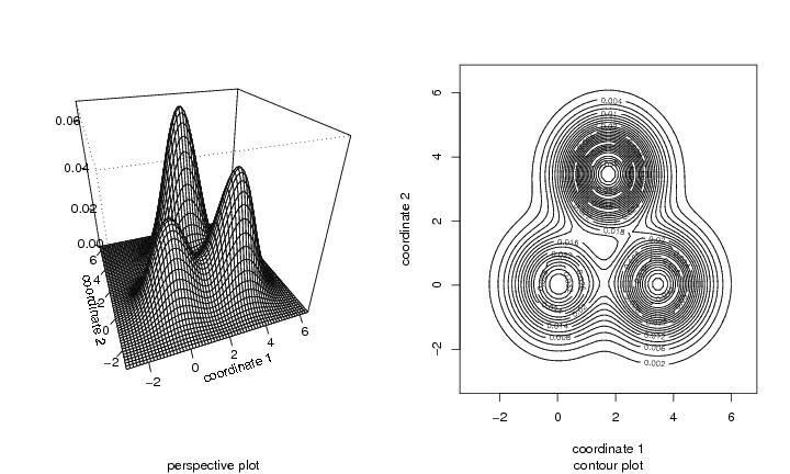
We consider the density shown in 2D three-modal density and generate a sample of size 200 from this density.
dendat<-sim.data(n=200,seed=5,type="mulmod")
We visualize a scale of kernel estimates. We calculate the sequence of estimates using the function ``lstseq.kern''.
h1<-0.85                    # the lowest h-value
h2<-2.3                     # the upper h-value
lkm<-100                    # number of estimates
base<-10                    # logarithmic spacing
hseq<-hgrid(h1,h2,lkm,base) # vector of h values
N<-c(30,30)                 # the size of the grid

estiseq<-lstseq.kern(dendat,hseq,N,kernel="epane",lstree=TRUE)
We make a mode graph from the sequence of kernel estimates.
mt<-modegraph(estiseq,hseq)
plotmodet(mt,coordi=1)
plotmodet(mt,coordi=2)
We make a map of branches from the sequence of kernel estimates.
bm<-branchmap(estiseq)
plotbranchmap(bm)
We plot the scale and shape visualization table.
scaletable(estiseq,shift=0.1,ptext=0.001,ptextst=0.3,
           bm=bm,levnum=NULL)