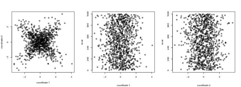
We generate and visualize the data with 4 extensions (cross).
dendat<-sim.data(n=1000,seed=1,type="cross")
We use function ``leafsfirst'' to calculate a tail tree. This function implements the algorithm LeafsFirst. We use resolution threshold rho=0.65.
rho<-0.65                             # resolution threshold
tt<-leafsfirst(dendat=dendat,rho=rho) # tail tree
We make parallel tail tree plots. We use the option ``modelabel'' to suppress the labeling of the modes. This makes the plotting faster.
plotbary(tt)                         #coordinate 1
plotbary(tt,coordi=2,modelabel=TRUE) #coordinate 2
We make a tail frequency plot with function ``plotvolu''.
plotvolu(tt)
We make a scatter plot where the segmentation is shown
ts<-tree.segme(tt)
plot(dendat,col=ts)