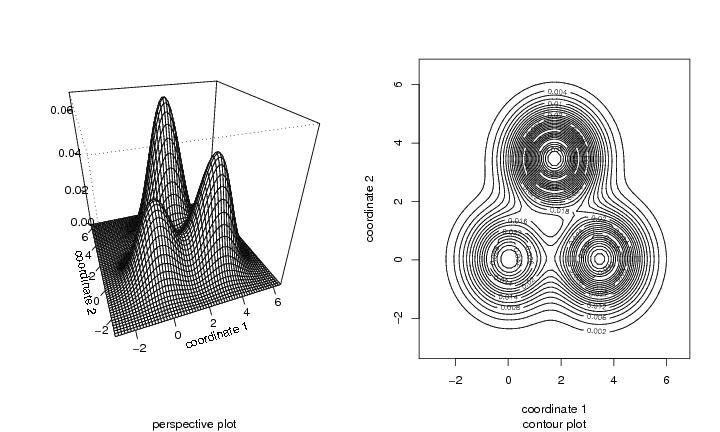
We give a code for drawing perspective plots and contour plots with the package "denpro". First we calculate a piecewise constant function.
N<-c(60,60)                       # size of the grid
pcf<-sim.data(N=N,type="mulmod")  # piecewise constant function
We use function ``draw.pcf'' to find the z-matrix and the x-coordinate and the y-coordinate, and then use R functions ``persp'' and ``contour'' to draw the function. These commands reproduce 2D three-modal density.
dp<-draw.pcf(pcf)
persp(dp$x,dp$y,dp$z,theta=-20,phi=30)
contour(dp$x,dp$y,dp$z,nlevels=25)
Function ``slicing'' constructs a slice of the function. First we calculate a 1D slice of the 2D function.
pcf.sl<-slicing(pcf,vecci=0)
In the 1D case we use the ``plot'' command to draw the function.
dp<-draw.pcf(pcf.sl)
plot(dp$x,dp$y,type="l")
Next we plot a 2D slice of a 3D function. The function has a Gaussian copula and Student marginals.
N<-c(26,26,26)  # choose the grid size
copula<-"gauss"
margin<-"student"
b<-4
support<-c(-b,b,-b,b,-b,b)
r<-0.5       # parameter of the copula
t<-c(2,2,2)  # degreeds of freedom for the student margin
pcf<-pcf.func(copula,N,marginal=margin,support=support,r=r,t=t)
The slice is defined as g(x1,x2)=f(x1,x2,0).
pcf.sl<-slicing(pcf,d1=1,d2=2,vecci=0)
dp<-draw.pcf(pcf.sl)
persp(dp$x,dp$y,dp$z,theta=30,phi=30)