Introduction

Figure 1

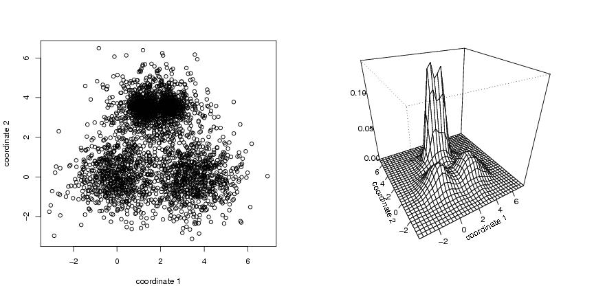
seed<-5
n<-3000
dendat<-sim.data(n=n,seed=seed,type="peaks")

h<-0.3
N<-c(40,40) 
bar<-pcf.kern(dendat,h,N) 
pnum<-N
deb<-draw.pcf(bar,corona=0,pnum=pnum)

# left frame
plot(dendat,xlab="coordinate 1",ylab="coordinate 2")

# right frame
persp(deb$x,deb$y,deb$z,theta=-25,phi=25,
xlab="coordinate 1",ylab="coordinate 2",zlab="",ticktype="detailed")

Figure 2

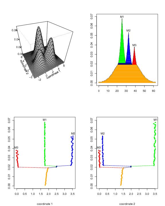
pcf<-sim.data(N=c(40,40),type="mulmod")

dp<-draw.pcf(pcf,pnum=c(40,40))

lst<-leafsfirst(pcf)

td<-treedisc(lst,pcf,ngrid=80)

# 1st frame
  phi<-35
  theta<--30
  persp(dp$x,dp$y,dp$z,phi=phi,theta=theta,ticktype="detailed", 
  xlab="coordinate 1 ",ylab="coordinate 2",zlab="")

# 2nd frame
  plotvolu(td,colo=TRUE,ptext=0.002,modelabel=TRUE) 

# 3rd frame
  plotbary(td,ptext=0.003,modelabel=TRUE) 

# 4th frame
  plotbary(td,coordi=2,ptext=0.003,modelabel=TRUE)

Figure 3

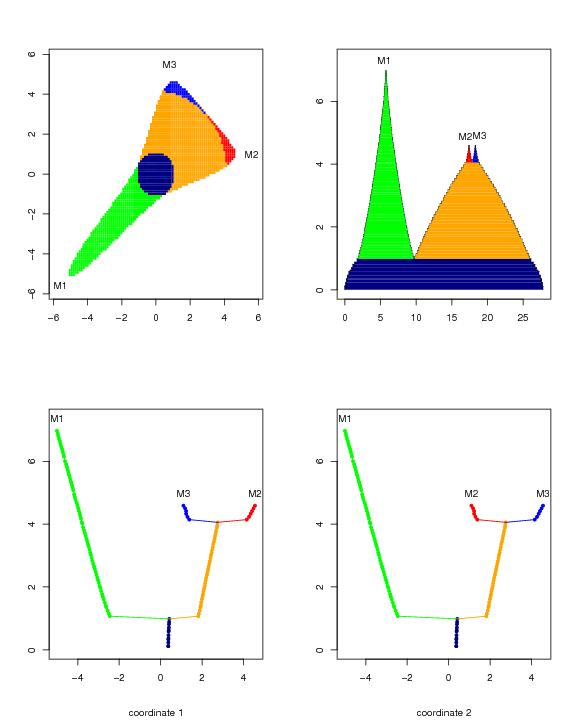
func<-"clayton"
N<-c(100,100) 
marginal<-"student"
yla<-5.8
ala<--yla
support<-c(ala,yla,ala,yla)
g<-4 
t<-c(4,4)

pcf<-pcf.func(func,N,support=support,marginal=marginal,g=g,t=t)

dp<-draw.pcf(pcf)

st.big<-leafsfirst(pcf,refe=c(0,0),propor=0.005)
st<-treedisc(st.big,pcf,ngrid=80)

paletti<-c("red","blue","green",
 "orange","navy","darkgreen",
 "orchid","aquamarine","turquoise",
 "pink","violet","magenta","chocolate","cyan",
 colors()[50:657],colors()[50:657])

st.big2<-prunemodes(st.big,modenum=3)
ts<-tree.segme(st.big2,pcf=pcf,paletti=paletti)

# 1st frame
  draw.levset(pcf,propor=0.005,col=ts)
  text(-5.6,-5.6,"M1")
  text(5.6,1.0,"M2")
  text(0.8,5.5,"M3")  

# 2nd frame
  plotvolu(st,modelabel=FALSE,colo=TRUE,ptext=0.4)  #,proba=TRUE,
  text(5.5,7.3,"M1")
  text(16.9,4.9,"M2")
  text(18.9,4.9,"M3")

# 3rd frame
  plotbary(st,modelabel=TRUE,ptext=0.4)

# 4th frame
  plotbary(st,modelabel=TRUE,coordi=2,ptext=0.4)

Figure 4

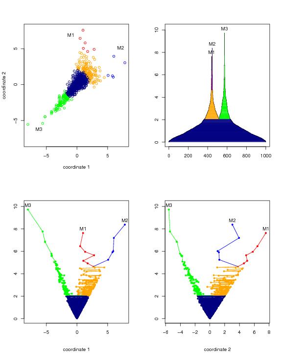
seed<-2
n<-1000

library(copula)
family="clayton"
g<-4 
c.cop<-archmCopula(family, param=g, dim=2)
set.seed(seed)
dendat<-rcopula(c.cop, n=n)
t<-c(4,4)
dendat<-qt(dendat,df=t)

rl<-min(dendat)
ru<-max(dendat)
rho<-1.4
tt<-leafsfirst(dendat=dendat,rho=rho)

paletti<-c("red","blue","green",
 "orange","navy","darkgreen",
 "orchid","aquamarine","turquoise",
 "pink","violet","magenta","chocolate","cyan",
 colors()[50:657],colors()[50:657])

ts<-tree.segme(tt,paletti=paletti)

# 1st frame
   plot(dendat,col=ts,
        xlim=c(rl,ru),ylim=c(rl,ru),
        xlab="coordinate 1",ylab="coordinate 2")
   text(-6.2,-6.2,"M3")
   text(7.1,5.1,"M2")
   text(-1.0,6.9,"M1")

# 2nd frame
   plotvolu(tt,modelabel=TRUE,colo=TRUE,ptext=0.4)

# 3rd frame
   plotbary(tt,coordi=1,modelabel=TRUE,ptext=0.4)
 
# 4th frame
   plotbary(tt,coordi=2,modelabel=TRUE,ptext=0.4)