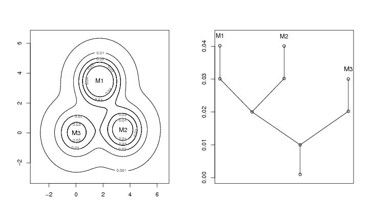
N<-c(64,64)
pcf<-sim.data(N=N,type="mulmod")

# Note: the calculation can take a long time
lst<-leafsfirst(pcf)

pn<-60
dp<-draw.pcf(pcf,pnum=c(pn,pn))

rad<-c(0.001,0.010,0.020,0.030,0.040)
lst.redu<-treedisc(lst,pcf,r=rad)

mc<-modecent(lst.redu)
radgrid<-lst.redu$level
roundrad<-round(radgrid,digits=3)

# frame 1
  contour(dp$x,dp$y,dp$z,levels=roundrad)
  text(mc[1,1],mc[1,2],"M1")
  text(mc[2,1],mc[2,2],"M2")
  text(mc[3,1],mc[3,2],"M3")

# frame 2
  plottree(lst.redu,ptext=0.003,colo=TRUE)
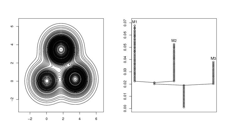
N<-c(64,64)
pcf<-sim.data(N=N,type="mulmod")

# Note: the calculation can take a long time
lst<-leafsfirst(pcf)

pn<-60
dp<-draw.pcf(pcf,pnum=c(pn,pn))

ngrid<-60
lst.redu<-treedisc(lst,pcf,ngrid=ngrid)
radgrid<-lst.redu$level
roundrad<-round(radgrid,digits=3)

# frame 1
  contour(dp$x,dp$y,dp$z,levels=roundrad,drawlabels=FALSE)

# frame 2
  plottree(lst.redu,ptext=0.003,colo=TRUE)
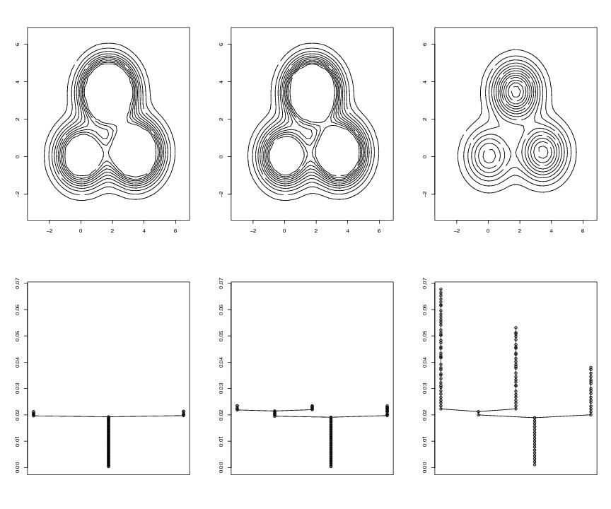
N<-c(40,40)
pcf<-sim.data(N=N,type="mulmod")
dp<-draw.pcf(pcf,pnum=N)

lenni<-length(pcf$value)
or<-order(pcf$value)
sequ<-c(1275,1325,lenni-1)
maxi<-max(pcf$value)

# frame 1
i<-1
ind<-sequ[i]
pcfcur<-pcf
pcfcur$value[or[(ind+1):lenni]]<-pcf$value[or[ind]]
dp<-draw.pcf(pcfcur,pnum=N)
lst<-leafsfirst(pcfcur)
lst2<-treedisc(lst,pcfcur,ngrid=60)
nodes<-length(lst2$parent)
contour(dp$x,dp$y,dp$z,xlab="",ylab="",labels="",nlevels=floor(nodes/6))

# frame 4
plottree(lst2,modelabel=FALSE,ylim=c(0,maxi))

# frame 2
i<-2
ind<-sequ[i]
pcfcur<-pcf
pcfcur$value[or[(ind+1):lenni]]<-pcf$value[or[ind]]
dp<-draw.pcf(pcfcur,pnum=N)
lst<-leafsfirst(pcfcur)
lst2<-treedisc(lst,pcfcur,ngrid=60)
nodes<-length(lst2$parent)
contour(dp$x,dp$y,dp$z,xlab="",ylab="",labels="",nlevels=floor(nodes/6))

# frame 5
plottree(lst2,modelabel=FALSE,ylim=c(0,maxi))

# frame 3
i<-3
ind<-sequ[i]
pcfcur<-pcf
pcfcur$value[or[(ind+1):lenni]]<-pcf$value[or[ind]]
dp<-draw.pcf(pcfcur,pnum=N)
lst<-leafsfirst(pcfcur)
lst2<-treedisc(lst,pcfcur,ngrid=60)
nodes<-length(lst2$parent)
contour(dp$x,dp$y,dp$z,xlab="",ylab="",labels="",nlevels=floor(nodes/6))

# frame 6
plottree(lst2,modelabel=FALSE,ylim=c(0,maxi))
n<-200
seed<-5
dendat<-sim.data(type="mulmod",n=n,seed=seed)

N<-c(64,64)
h<-0.28   #0.5
pcf<-pcf.kern(dendat,h,N,kernel="gauss")

# warning: calculation can take a long time
lst<-leafsfirst(pcf)
lst.redu<-treedisc(lst,pcf,ngrid=120)

pn<-45
dp<-draw.pcf(pcf,pnum=c(pn,pn))
mc<-modecent(lst.redu)
radgrid<-lst.redu$level

# frame 1
  persp(dp$x,dp$y,dp$z,phi=35,theta=20,ticktype="detailed",
  xlab="",ylab="",zlab="")

# frame 2
  contour(dp$x,dp$y,dp$z,nlevels=30,drawlabels=FALSE)
  for (i in 1:dim(mc)[1]) text(mc[i,1],mc[i,2],paste("M",as.character(i)))

# frame 3
  plottree(lst.redu,ptext=0.003,colo=TRUE)
d<-2
mixnum<-5
M<-matrix(0,mixnum,d)
M[1,]<-c(0,0)
M[2,]<-c(5,0)
M[3,]<-c(0,5)
M[4,]<-c(5,5)
M[5,]<-c(2.5,2.5)
sig<-matrix(1,mixnum,d)
p<-c(-1,-1,1,1,2)
N<-c(40,40)

lowest<--10
pcf<-pcf.func("mixt",N,sig=sig,M=M,p=p,lowest=lowest)

dp<-draw.pcf(pcf,pnum=c(40,40))

lst<-leafsfirst(pcf,lowest="gene")
ngrid<-100
lst.redu<-treedisc(lst,pcf,ngrid=ngrid,lowest="gene")

pcf.lower<-pcf
pcf.lower$value<--pcf$value
lst.lower<-leafsfirst(pcf.lower,lowest="gene")
ngrid<-99
lst.lower.redu<-treedisc(lst.lower,pcf.lower,ngrid=ngrid,lowest="gene")
lst.lower.2<-lst.lower.redu
lst.lower.2$level<--lst.lower.redu$level

# frame 1
  persp(dp$x,dp$y,dp$z,phi=40,theta=-20,ticktype="detailed",
  xlab="",ylab="",zlab="")

# frame 2
  ptext<-0.03
  plottree(lst.redu,ptext=ptext,colo=FALSE,lowest="gene")

# frame 3
  symbo<-"L"
  ptext<--0.025
  ymargin<-0.04
  plottree(lst.lower.2,ptext=ptext,symbo=symbo,colo=FALSE,lowest="gene",
  ymargin=ymargin)
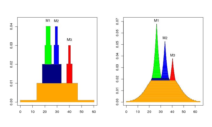
N<-c(64,64)
pcf<-sim.data(N=N,type="mulmod")

lst<-leafsfirst(pcf)

rad<-c(0.001,0.010,0.020,0.030,0.040)
lst.redu<-treedisc(lst,pcf,r=rad)

ngrid<-100
lst.redu2<-treedisc(lst,pcf,ngrid=ngrid)

# frame 1
 plotvolu(lst.redu,ptext=0.003,modelab=TRUE,colo=TRUE)

# frame 2
 plotvolu(lst.redu2,ptext=0.003,modelab=TRUE,colo=TRUE)

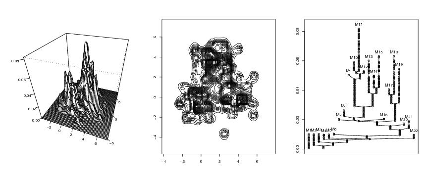
n<-200
seed<-5
dendat<-sim.data(type="mulmod",n=n,seed=seed)

N<-c(64,64)
h<-0.28   #0.5
pcf<-pcf.kern(dendat,h,N,kernel="gauss")

lst<-leafsfirst(pcf)
lst.redu<-treedisc(lst,pcf,ngrid=120)

pn<-45
dp<-draw.pcf(pcf,pnum=c(pn,pn))
mc<-modecent(lst.redu)
radgrid<-lst.redu$level

# frame 1
  persp(dp$x,dp$y,dp$z,phi=35,theta=20,ticktype="detailed",
  xlab="",ylab="",zlab="")

# frame 2
  plotvolu(lst.redu,ptext=0.003,colo=TRUE,modelabel=TRUE)
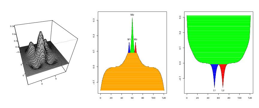
d<-2
mixnum<-5
M<-matrix(0,mixnum,d)
M[1,]<-c(0,0)
M[2,]<-c(5,0)
M[3,]<-c(0,5)
M[4,]<-c(5,5)
M[5,]<-c(2.5,2.5)
sig<-matrix(1,mixnum,d)
p<-c(-1,-1,1,1,2)
N<-c(80,80)

pcf<-pcf.func("mixt",N,sig=sig,M=M,p=p,lowest=-10)

dp<-draw.pcf(pcf,pnum=c(40,40))

lst<-leafsfirst(pcf,lowest="gene")
lst.redu<-treedisc(lst,pcf,ngrid=100,lowest="gene")

pcf.lower<-pcf
pcf.lower$value<--pcf$value
lst.lower<-leafsfirst(pcf.lower,lowest="gene")
lst.lower.redu<-treedisc(lst.lower,pcf.lower,ngrid=150,lowest="gene")
lst.lower.2<-lst.lower.redu
lst.lower.2$level<--lst.lower.redu$level

# frame 1
  persp(dp$x,dp$y,dp$z,phi=40,theta=-20,ticktype="detailed",
  xlab="",ylab="",zlab="")

# frame 2
  ptext<-0.02
  plotvolu(lst.redu,ptext=ptext,modelabel=TRUE,colo=TRUE,lowest="gene")

# frame 3
  symbo<-"L"
  ptext<-0.02
  ylim<-c(min(lst.lower.2$level)-ptext,max(pcf$value))
  plotvolu(lst.lower.2,ylim=ylim,ptext=-ptext,symbo=symbo,
  modelabel=TRUE,colo=TRUE,lowest="gene",upper=FALSE)

func<-"hat"
yla<-6;ala<--yla;support<-c(ala,yla,ala,yla)
a<-0.5
b<-1

N<-c(60,60)
pcf<-eval.func.dD(func,N,support=support,a=a,b=b)
dp<-draw.pcf(pcf,pnum=N)

lst<-leafsfirst(pcf)
lst.redu<-treedisc(lst,pcf,ngrid=150)

# frame 1
  persp(dp$x,dp$y,dp$z,phi=30,theta=30,
  ticktype="detailed",xlab="",ylab="",zlab="")

# frame 2
  plotvolu(lst.redu)
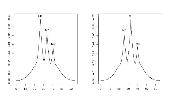
N<-c(64,64)
pcf<-sim.data(N=N,type="mulmod")

# Note: the calculation can take a long time
lst<-leafsfirst(pcf)

ngrid<-100
lst.redu2<-treedisc(lst,pcf,ngrid=ngrid)

# frame 1
 plotvolu(lst.redu2,ptext=0.003,modelab=TRUE)

# frame 2
 leimat<-c("M2","M1","M3")
 plotvolu(lst.redu2,ptext=0.003,modelab=TRUE,crit=c(-10,-1),leimat=leimat)

trans3d <- function(x,y,z, pmat) {
  tr <- cbind(x,y,z,1) %*% pmat
  list(x = tr[,1]/tr[,4], y= tr[,2]/tr[,4])
}

N<-c(64,64)
pcf<-sim.data(N=N,type="mulmod")

# Note: the calculation can take a long time
lst<-leafsfirst(pcf)

ngrid<-100
lst.redu2<-treedisc(lst,pcf,ngrid=ngrid)

pn<-40
dm<-draw.pcf(pcf,pnum=c(pn,pn))
persp(dm$x,dm$y,dm$z,theta=-50,phi=0)

pt<-lst.redu2
paletti<-c("red","blue","green",
 "orange","navy","darkgreen",
 "orchid","aquamarine","turquoise",
 "pink","violet","magenta","chocolate","cyan",
 colors()[50:100])
col<-colobary(pt$parent,paletti)

fb<-findbranch(pt$parent)
lenni<-length(fb$indicator)
nodepoint<-matrix(0,lenni,1)
laskuri<-0
for (i in 1:lenni){
    if (fb$indicator[i]==1){
          nodepoint[laskuri]<-i
          laskuri<-laskuri+1
    }
}
nodepoint<-nodepoint[1:(laskuri-1)]

# frame
 persp(dm$x,dm$y,dm$z,theta=-5,phi=10,
 xlab="",ylab="",zlab="",box=FALSE)->res

 x<-pt$center[1,]
 y<-pt$center[2,]
 z<-pt$level #-0.0025
 points(trans3d(x=x, y=y, z=z, pm = res),col=col,pch=16)

 a<-pt$center[1,nodepoint][1:2]
 b<-pt$center[2,nodepoint][1:2]
 c<-pt$level[nodepoint][1:2]
 lines(trans3d(x=a, y=b, z=c, pm = res), col="black", pch=16, lwd=2)

 a<-pt$center[1,nodepoint][3:4]
 b<-pt$center[2,nodepoint][3:4]
 c<-pt$level[nodepoint][3:4]
 lines(trans3d(x=a, y=b, z=c, pm = res), col="black", pch=16, lwd=2)
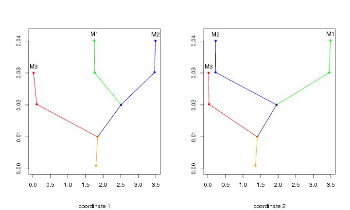
N<-c(64,64)
pcf<-sim.data(N=N,type="mulmod")

# Note: the calculation can take a long time
lst<-leafsfirst(pcf)

rad<-c(0.001,0.010,0.020,0.030,0.040)
lst.redu<-treedisc(lst,pcf,r=rad)

# frame 1
 plotbary(lst.redu,coordi=1,ptext=0.002,modlab=TRUE)

# frame 2
 plotbary(lst.redu,coordi=2,ptext=0.002,modlab=TRUE)
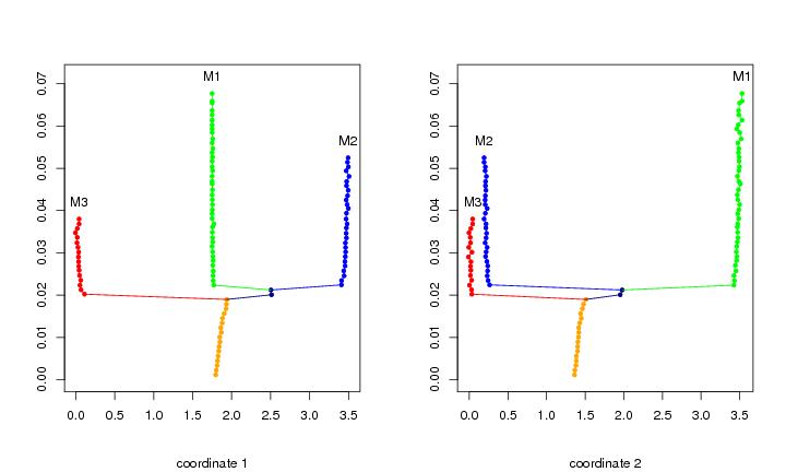
N<-c(64,64)
pcf<-sim.data(N=N,type="mulmod")

# Note: the calculation can take a long time
lst<-leafsfirst(pcf)

ngrid<-60
lst.redu<-treedisc(lst,pcf,ngrid=ngrid)

# frame 1
 plotbary(lst.redu,coordi=1,ptext=0.004,modlab=TRUE)

# frame 2
 plotbary(lst.redu,coordi=2,ptext=0.004,modlab=TRUE)
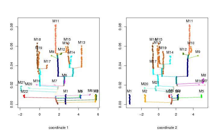
n<-200
seed<-5
dendat<-sim.data(type="mulmod",n=n,seed=seed)

N<-c(64,64)
h<-0.28
pcf<-pcf.kern(dendat,h,N,kernel="gauss")

lst<-leafsfirst(pcf)
lst.redu<-treedisc(lst,pcf,ngrid=120)

# frame 1
 plotbary(lst.redu,coordi=1,ptext=0.004,modlab=TRUE)

# frame 2
 plotbary(lst.redu,coordi=2,ptext=0.004,modlab=TRUE)
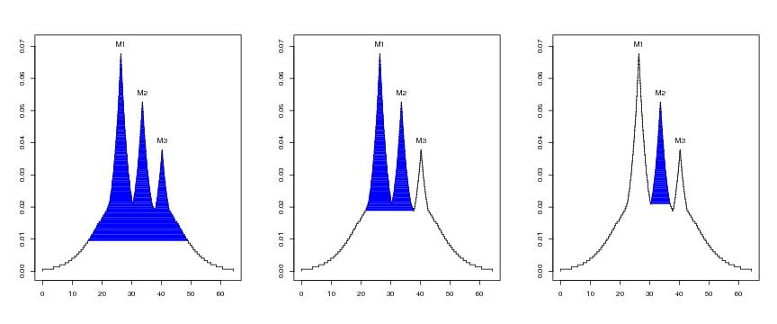
N<-c(64,64)
pcf<-sim.data(N=N,type="mulmod")

# Note: the calculation can take a long time
lst<-leafsfirst(pcf)

ngrid<-100
lst.redu2<-treedisc(lst,pcf,ngrid=ngrid)

fb<-findbranch(lst.redu2$parent)
#t(fb$indicator)

# frame 1
  plotvolu(lst.redu2,ptext=0.003,modelabel=TRUE,exmavisu=15)

# frame 2
  plotvolu(lst.redu2,ptext=0.003,modelabel=TRUE,exmavisu=29)

# frame 3
  plotvolu(lst.redu2,ptext=0.003,modelabel=TRUE,exmavisu=35)
d<-1
mnum<-2
D<-3
M<-matrix(0,mnum,d)
M[1]<-0
M[2]<-D
sig<-matrix(0,mnum,d)
sig[1]<-1
sig[2]<-1
p<-c(0.35,0.65)
support<-matrix(0,2,1)
mul<-3
support[1]<-min(M-mul*sig)
support[2]<-max(M+mul*sig)
N<-100
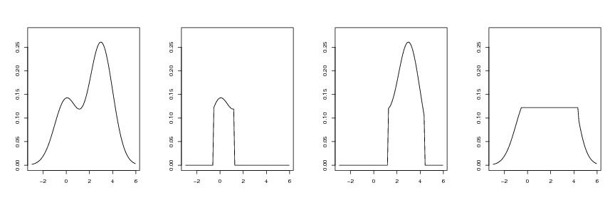
pcf<-pcf.func("mixt",N,sig=sig,M=M,p=p,support=support)
dp<-draw.pcf(pcf)
vasy<-matrix(0,length(dp$y),1)
vasy[28:47]<-dp$y[28:47]
oiky<-matrix(0,length(dp$y),1)
oiky[48:82]<-dp$y[48:82]
resty<-matrix(0,length(dp$y),1)
resty[1:27]<-dp$y[1:27]
resty[83:100]<-dp$y[83:100]
resty[28:82]<-dp$y[28]
# frame 1
yl<-0.28
plot(dp$x,dp$y,type="l",ylim=c(0,yl),xlab="",ylab="")
# frame 2
plot(dp$x,vasy,type="l",ylim=c(0,yl),xlab="",ylab="")
# frame 3
plot(dp$x,oiky,type="l",ylim=c(0,yl),xlab="",ylab="")
# frame 4
plot(dp$x,resty,type="l",ylim=c(0,yl),xlab="",ylab="")
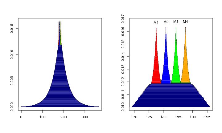
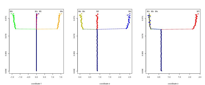
N<-c(32,32,32)
pcf<-sim.data(N=N,type="tetra3d")

# Warning: the calculation can take a long time
lst<-leafsfirst(pcf)

lst.redu<-treedisc(lst,pcf,ngrid=200)

# frame 1
  plotvolu(lst.redu,modelabel=FALSE,colo=TRUE)

# frame 2
  plotvolu(lst.redu,cutlev=0.010,ptext=0.00045,colo=TRUE,modelabel=TRUE)
N<-c(32,32,32)
pcf<-sim.data(N=N,type="tetra3d")

# Warning: the calculation can take long
lst<-leafsfirst(pcf)

lst.redu<-treedisc(lst,pcf,ngrid=200)

mc<-modecent(lst.redu)
y=rep(0.017,4)
leimat<-c("M2","M3","M4","M1")

x1<-mc[,1]
x1[1]<-x1[1]-0.15
x1[4]<-x1[4]+0.1

x2<-mc[,2]
x2[2]<-x2[2]-0.1
x2[3]<-x2[3]+0.1

x3<-mc[,3]
x3[1]<-x3[1]-0.05
x3[2]<-x3[2]+0.15
x3[3]<-x3[3]+0.35

# frame 1
  plotbary(lst.redu,coordi=1,ptext=0.0006)
  text(x1,y,labels=leimat)

# frame 2
  plotbary(lst.redu,coordi=2,ptext=0.0006)
  text(x2,y,labels=leimat)

# frame 3
  plotbary(lst.redu,coordi=3,ptext=0.0006)
  text(x3,y,labels=leimat)
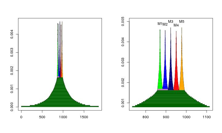
N<-c(16,16,16,16)
pcf<-sim.data(N=N,type="penta4d")

# Warning: the calculation can take long
lst<-leafsfirst(pcf)

lst.redu<-treedisc(lst,pcf,ngrid=100)

# frame 1
   plotvolu(lst.redu,modelabel=FALSE,colo=TRUE)

# frame 2
   plotvolu(lst.redu,cutlev=0.0008,ptext=0.0003,colo=TRUE,modelabel=TRUE)
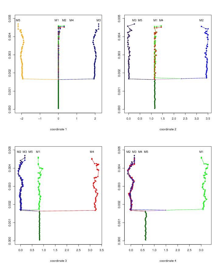
N<-c(16,16,16,16)
pcf<-sim.data(N=N,type="penta4d")

# Warning: the calculation can take long
lst<-leafsfirst(pcf)

lst.redu<-treedisc(lst,pcf,ngrid=100)

mc<-modecent(lst.redu)
y=rep(0.0049,5)
leimat<-c("M4","M2","M1","M5","M3")

x1<-mc[,1]
x1[3]<-x1[3]-0.4
x1[1]<-x1[1]+0.4

x2<-mc[,2]
x2[3]<-x2[3]-0.25
x2[4]<-x2[4]+0.25

x3<-mc[,3]
x3[2]<-x3[2]-0.25
x3[4]<-x3[4]+0.25

x4<-mc[,4]
x4[2]<-x4[2]-0.25
x4[1]<-x4[1]+0.25
x4[4]<-x4[4]+0.5

# frame 1
  plotbary(lst.redu,coordi=1,ptext=0.0003) #,col=col,collines=col)
  text(x1,y,labels=leimat)

# frame 2
  plotbary(lst.redu,coordi=2,ptext=0.0003)
  text(x2,y,labels=leimat)

# frame 3
  plotbary(lst.redu,coordi=3,ptext=0.0003)
  text(x3,y,labels=leimat)

# frame 4
  plotbary(lst.redu,coordi=4,ptext=0.0003)
  text(x4,y,labels=leimat)
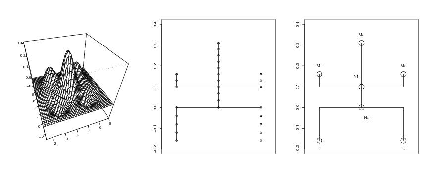
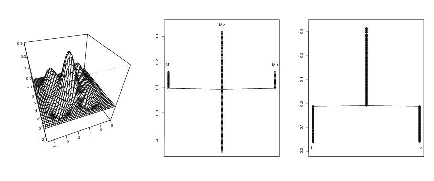
d<-2
mixnum<-5
M<-matrix(0,mixnum,d)
M[1,]<-c(0,0)
M[2,]<-c(5,0)
M[3,]<-c(0,5)
M[4,]<-c(5,5)
M[5,]<-c(2.5,2.5)
sig<-matrix(1,mixnum,d)
p<-c(-1,-1,1,1,2)
N<-c(40,40)

lowest<--1
pcf<-pcf.func("mixt",N,sig=sig,M=M,p=p,lowest=lowest)
dp<-draw.pcf(pcf,pnum=c(40,40))

# frame 1
persp(dp$x,dp$y,dp$z,phi=40,theta=-20,ticktype="detailed",
xlab="",ylab="",zlab="")

# frame 2
plot(x="",y="",xlim=c(0,1),ylim=c(-0.2,0.4),xlab="",ylab="", xaxt="n")

points(0.1,0.16)  #M1
points(0.5,0.31)  #M2
points(0.9,0.16)  #M3
points(0.5,-0.0)
points(0.1,-0.16) #L1
points(0.9,-0.16) #L2

segments(0.1,0.1,0.1,0.16)
segments(0.5,-0.0,0.5,0.31)
segments(0.1,0.1,0.9,0.1)
segments(0.9,0.1,0.9,0.16)
segments(0.1,-0.0,0.9,-0.0)
segments(0.1,-0.0,0.1,-0.16)
segments(0.9,-0.0,0.9,-0.16)

step<-(0.16-0.1)/2
for (i in 0:2) points(0.1,0.1+i*step)
for (i in 0:2) points(0.9,0.1+i*step)
for (i in 1:7) points(0.5,0.1+i*step)

step<-(0.1--0.0)/3
for (i in 1:3) points(0.5,-0.0+i*step)
step<-(-0.0--0.16)/4
for (i in 1:4) points(0.1,-0.16+i*step)
step<-(-0.0--0.16)/4
for (i in 1:4) points(0.9,-0.16+i*step)

# frame 3
plot(x="",y="",xlim=c(0,1),ylim=c(-0.2,0.4),xlab="",ylab="", xaxt="n")

cex<-3
points(0.1,0.16,cex=cex)  #M1
points(0.5,0.31,cex=cex)  #M2
points(0.9,0.16,cex=cex)  #M3
points(0.5,0.1,cex=cex)
points(0.5,-0.0,cex=cex)
points(0.1,-0.16,cex=cex) #L1
points(0.9,-0.16,cex=cex) #L2

text(0.1,0.20,"M1")
text(0.5,0.35,"M2")
text(0.9,0.20,"M3")
text(0.45,0.15,"N1")
text(0.55,-0.05,"N2")
text(0.1,-0.20,"L1")
text(0.9,-0.20,"L2")

segments(0.1,0.1,0.1,0.16)
segments(0.5,-0.0,0.5,0.31)
segments(0.1,0.1,0.9,0.1)
segments(0.9,0.1,0.9,0.16)
segments(0.1,-0.0,0.9,-0.0)
segments(0.1,-0.0,0.1,-0.16)
segments(0.9,-0.0,0.9,-0.16)