Chapter 7: Scales of density estimates

Figure 1

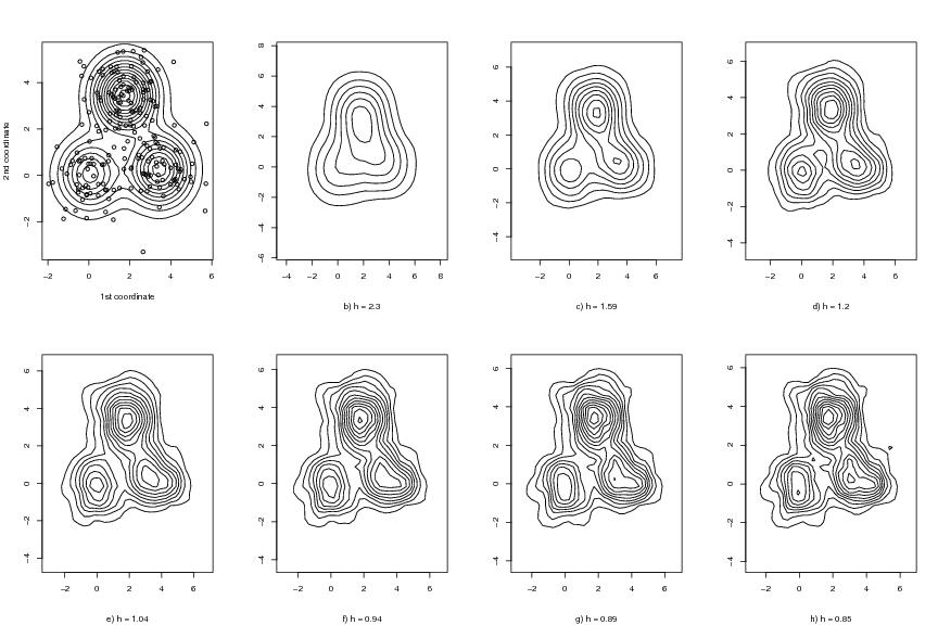
dendat<-sim.data(n=200,seed=5,type="mulmod")

h1<-0.85
h2<-2.3
lkm<-100
base<-10
hseq<-hgrid(h1,h2,lkm,base)
N<-c(30,30)   

# Warning: the calculation can take a long time
estiseq<-lstseq.kern(dendat,hseq,N,lstree=TRUE,level=0.1,kernel="epane") 

egf<-sim.data(N=N,type="mulmod")
dpf<-draw.pcf(egf)

hind<-c(1,20,40,55,70,85,100)
for (i in 1:7){
   pcf<-estiseq$pcfseq[[hind[i]]]
   if (i==1) pcflist<-list(pcf)
   else pcflist<-c(pcflist,list(pcf))
}

lapeli<-c("b)","c)","d)","e)","f)","g)","h)")

# frame 1
plot(dendat,xlab="1st coordinate",ylab="2nd coordinate")
contour(dpf$x,dpf$y,dpf$z,drawlabels=FALSE,add=TRUE)

# frames 2-8
for (i in 1:length(hind)){
   pcf<-pcflist[[i]]
   dp<-draw.pcf(pcf)
   contour(dp$x,dp$y,dp$z,drawlabels=FALSE) 
   title(sub=paste(lapeli[i],"h =",
   as.character(round(estiseq$hseq[hind[i]],digits=2))))
}

Figure 2

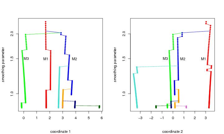
dendat<-sim.data(n=200,seed=5,type="mulmod")

h1<-0.85
h2<-2.3
lkm<-100
base<-10
hseq<-hgrid(h1,h2,lkm,base)
N<-c(30,30)   

# Warning: the calculation can take a long time
estiseq<-lstseq.kern(dendat,hseq,N,lstree=TRUE,level=0.1,kernel="epane") 

mt<-modegraph(estiseq)

# frame 1
plotmodet(mt,coordi=1,ylab="smoothing parameter")  
text(0.2,1.5,"M3")
text(1.7,1.5,"M1")
text(3.9,1.5,"M2")

# frame 2
plotmodet(mt,coordi=2,ylab="smoothing parameter")  
text(-0.7,1.5,"M3")
text(2.8,1.5,"M1")
text(0.9,1.5,"M2")

Figure 3

dendat<-sim.data(n=200,seed=5,type="mulmod")

h1<-0.85
h2<-2.3
lkm<-100
base<-10
hseq<-hgrid(h1,h2,lkm,base)
N<-c(30,30)   

# Warning: the calculation can take a long time
estiseq<-lstseq.kern(dendat,hseq,N,lstree=TRUE,level=0.1,kernel="epane") 

ii<-2

h<-estiseq$hseq[hind[ii]]
pcf<-estiseq$pcfseq[[hind[ii]]]
lst<-estiseq$lstseq[[hind[ii]]]

td<-treedisc(lst,pcf,30)

fb<-findbranch(td$parent,colo="blue",pch=24)

em<-excmas(td)
em<-em/em[1]
emr<-matrix("",length(em),1) 
for (i in 1:length(fb$indicator)){
   if (fb$indicator[i]==1){ 
         emr[i]<-round(10000*em[i])/10000
         fb$colovec[td$parent[i]]<-"red1"   
         fb$pchvec[td$parent[i]]<-22 
   }
}

bm<-branchmap(estiseq)

hindeksi<-101-hind[ii]

x<-bm$level
y<-bm$z[,hindeksi]
alku<-(dim(bm$z)[1]-1)*hindeksi+2
loppu<-alku+dim(bm$z)[1]-1
col<-bm$col[alku:loppu]
col[length(col)]<-"white"
col[length(col)-1]<-"white"

node1<-27
node2<-39
node3<-57

# frame 1
plottree(td,ptext=0.003,info=emr,xmarginright=0.25,xmarginleft=0.05,
infopos=-0.3,infolift=0.0005,col=fb$colovec,pch=fb$pchvec,cex=1.5,nodemag=2,
cex.axis=1.5,ylab="level",cex.lab=1.5)

# frame 2
plot(x,y,col=col,lty=1,xlab="level",ylab="excess mass",pch=19,
cex.lab=1.5,cex.axis=1.5)  
segments(x[node1+1],y[node1],x[node1+1],y[node1+1],lty=1)
segments(x[node2+1],y[node2],x[node2+1],y[node2+1])
segments(x[node3+1],y[node3],x[node3+1],0)

Figure 4

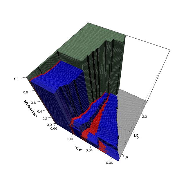
dendat<-sim.data(n=200,seed=5,type="mulmod")

h1<-0.85
h2<-2.3
lkm<-100
base<-10
hseq<-hgrid(h1,h2,lkm,base)
N<-c(30,30)   

# Warning: the calculation can take a long time
estiseq<-lstseq.kern(dendat,hseq,N,lstree=TRUE,level=0.1,kernel="epane") 

bm<-branchmap(estiseq)

# frame 
  plotbranchmap(bm)