Chapter 4: Level set trees. Code

We show how to make a volume plot and a barycenter plot. We calculate level set trees with the algorithm LeafsFirst, which is implemented in function ``leafsfirst''. This function takes as an argument a picewise constant function object.

The multimodal 2D example

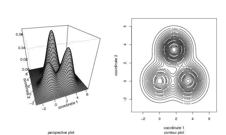
We consider the density shown in the 2D three-modal density, and calculate first a piecewise constant function object representing this function, and then calculate the level set tree.

N<-c(35,35)                      # size of the grid
pcf<-sim.data(N=N,type="mulmod") # piecewise constant function
lst.big<-leafsfirst(pcf)         # level set tree

We may make the volume plot with the command ``plotvolu(lst)''. However, it is faster first to prune the level set tree, and then plot the reduced level set tree. Function ``treedisc'' takes as the first argument a level set tree, as the second argument the original piecewise constant function, and the 3rd argument ``ngrid'' gives the number of levels in the pruned level set tree. We try the number of levels ngrid=100.

lst<-treedisc(lst.big,pcf,ngrid=100)

Now we may make a volume plot with the function ``plotvolu''.

plotvolu(lst)

We draw barycenter plots with the function ``plotbary''.

plotbary(lst,coordi=2)  # 2nd coordinate

Remark. One may make a perspective plot and contour plot with the commands of Chapter 2.

Remark. We may find the number and the location of the modes with the ``modecent'' function, which takes as argument a level set tree. Function ``locofmax'' takes as argument a piecewise constant function and calculates the location of the maximum.

modecent(lst)
locofmax(pcf)

The 3D tetrahedron example

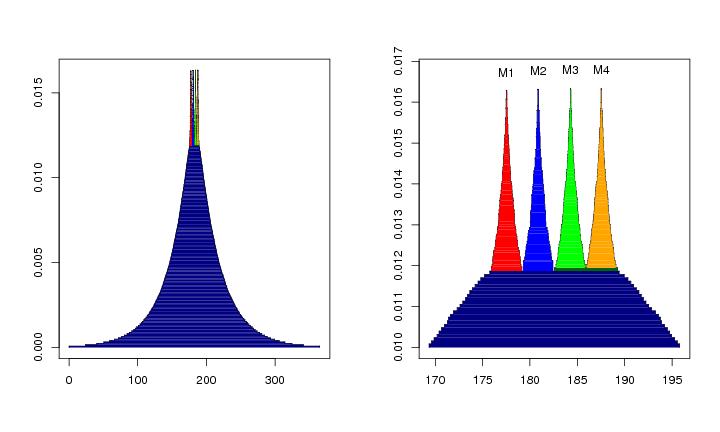
We consider the 3-dimensional example. The calculation is much more time consuming this time.

N<-c(32,32,32)                    # the size of the grid
pcf<-sim.data(N=N,type="tetra3d") # piecewise constant function
lst.big<-leafsfirst(pcf)             # level set tree
lst<-treedisc(lst.big,pcf,ngrid=200) # pruned level set tree

plotvolu(lst,modelabel=FALSE)        # volume plot
plotvolu(lst,cutlev=0.010,ptext=0.00045,colo=TRUE) # zooming

coordi<-1                   # coordinate, coordi = 1, 2, 3
plotbary(lst,coordi=coordi,ptext=0.0006) # barycenter plot

This time we have used parameter ``cutlev'' to make a zoomed volume plot. When this parameter is given, then only the part of the level set tree is shown which is above the value ``cutlev''. Typically it is better to zoom in to the volume plot by cutting the tails of the volume function away. This is achieved by the parameter ``xlim''. We may us for example the following command to make a ``vertically zoomed'' volme plot.

plotvolu(lst,xlim=c(140,220),ptext=0.00045,
         colo=TRUE,modelabel=FALSE)

Additional parameters which we have used are the ``modelabel'', which is used to suppress the plotting of the mode labels, ``ptext'', which lifts the mode labels with the given amount, and ``colo'', which colors the graph of the volume function to make a comparison with the barycenter plots easier.

The 4D pentahedron example

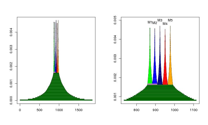
We consider the 4-dimensional example.

N<-c(16,16,16,16)  
pcf<-sim.data(N=N,type="penta4d")
lst.big<-leafsfirst(pcf)
lst<-treedisc(lst.big,pcf,ngrid=100)

plotvolu(lst,modelabel=F)  # volume plot
plotvolu(lst,cutlev=0.0008,ptext=0.00039,colo=TRUE) # zooming

coordi<-1               # coordinate, coordi = 1, 2, 3, 4
plotbary(lst,coordi=coordi,ptext=0.0003) # barycenter plot