We give instructions to make shape plots and a location plot. We calculate shape trees with the algorithm LeafsFirst, which is implemented in function ``leafsfirst''.
We consider the Fox density, and calculate first a piecewise constant function object representing this function. Code of Chapter 2 gives the commands to make a perspective plot and a contour plot from a piecewise constant function.
N<-c(100,100)                  # size of the grid
pcf<-sim.data(N=N,type="fox")  # piecewise constant function
We calculate the shape tree for the level set with level 0.002, when the reference point is at the origin.
lev<-0.002                       # level of the level set
refe<-c(0,0)                     # reference point
st.big<-leafsfirst(pcf,lev,refe) # shape tree
We prune the level set tree to contain 33 levels.
st<-treedisc(st.big,pcf,ngrid=33)
Now we may plot the radius function and location plot. We give here the basic forms of the commands but in later examples we apply more tuning parameters.
plotvolu(st)          # radius plot
plotbary(st,coordi=1) # location plot, 1st coordinate
We make a tail probability plot. We use the shape tree ``st'' calculated above.
plotvolu(st,proba=TRUE)
To make a probability content plot we need to calculate a modified level set tree.
st.proba<-leafsfirst(pcf,lev,refe,levmet="proba")
st2<-treedisc(st.proba,pcf,ngrid=33)
plotvolu(st2)
We consider the skewed Gaussian density. First we calculate the piecewise constant function object.
func<-"skewgauss"
N<-c(100,100)         # the size of the grid
support<-c(-6,2,-6,2) # the range of the evaluation
mu<-c(0,0)            # the center
sig<-c(3,1)           # marginal standard deviations
alpha<-c(6,0)         # the skeweness parameter
theta<--3*pi/4        # we rotate the function

pcf<-pcf.func(func,N,support=support,mu=mu,sig=sig,
              alpha=alpha,theta=theta)
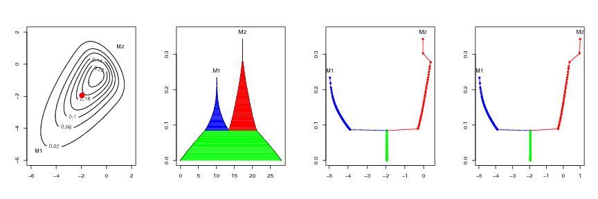
We calculate a shape tree of piecewise constant function ``pcf''. We use the 7% level set. The p%-level set is the level set with level p times the maximum of f. This level is calculated from ``value'' component of ``pcf''. When we do not give a reference point as an argument to the call of function ``leafsfirst'', then the location of the maximum is used as a reference point.
st.big<-leafsfirst(pcf,propor=0.07)# shape tree
st<-treedisc(st.big,pcf,ngrid=26)  # pruned shape tree
We make a radius plot and location plot. We use parameter ``ptext'' to lift the positions of mode labels, and use parameter ``colo'' to color the graph of the radius function.
plotvolu(st,ptext=0.2,colo=TRUE)  # radius plot
plotbary(st,ptext=0.2,coordi=1)   # location plot
Next we change the reference point to be the barycenter of the level set. The barycenter of the level set is calculated simultaneously when the shape tree is calculated, and thus we have the barycenter as the ``bary'' component of ``st.big''.
refe<-st.big$bary               # barycenter as reference point
st.bary<-leafsfirst(pcf,lev,refe)  # shape tree
st<-treedisc(st.bary,pcf,ngrid=40) # pruned shape tree
plotvolu(st,ptext=0.2,colo=TRUE)   # radius plot
plotbary(st,ptext=0.2,coordi=1)    # location plot
Sometimes a radius function has spurious modes, which one would like to prune away. We use the function ``prunemodes'' for pruning away the modes with the smallest excess mass. Below ``st100'' has 15 modes and especially the location plot looks messy. We prune 13 modes away leaving the 2 main modes left. We may calculate the number and location of the modes with command ``modecent(st100)''. With the mode pruning we may have more granularity in the radius function, by choosing parameter ``ngrid'' large.
st100<-treedisc(st.bary,pcf,ngrid=100)#st100 has spurious modes
plotvolu(st100,ptext=0.2,colo=TRUE)   #radius plot
plotbary(st100,ptext=0.2,coordi=1)    #location plot

st<-prunemodes(st100,modenum=2)     # mode pruning
plotvolu(st,ptext=0.2,colo=TRUE)    # radius plot
plotbary(st,ptext=0.2,coordi=1)     # location plot