We apply function ``sim.data'', to generate a sample of size 200 from the 2D three-modal density.
dendat<-sim.data(n=200,seed=5,type="mulmod")
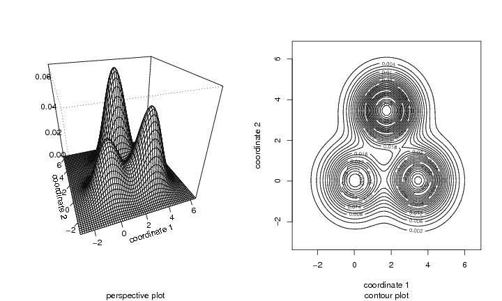
First we calculate the kernel estimate with the Bartlett-Epanechnikov kernel and with smoothing parameter h=1.4. Function ``pcf.kern'' gives the estimate as a piecewise constant function object.
h<-1.4       # smoothing parameter
N<-c(60,60)  # the size of the grid
pcf<-pcf.kern(dendat,h,N,kernel="epane")

dp<-draw.pcf(pcf)
persp(dp$x,dp$y,dp$z,theta=-20,phi=30)
Second we calculate the kernel estimate with the standard Gaussian kernel and with smoothing parameter h=0.8.
h<-0.8
pcf<-pcf.kern(dendat,h,N,kernel="gauss")

dp<-draw.pcf(pcf)
persp(dp$x,dp$y,dp$z,theta=-20,phi=30)
Code of Chapter 2 gives the commands to make a perspective plot and a contour plot from a piecewise constant function. Code of Chapter 4 and Code of Chapter 5 give commands for using level set trees and shape trees to visualize kernel estimates.